SSE models
In this tutorial you fit BiSSE, a state-dependent speciation and extinction model, to habitat_binary. You read its diagnostics, then try the MuSSE, QuaSSE and hidden-state cards. The small example is for learning the controls and the checks, not for testing a hypothesis.
The bundled example is synthetic. Its values are invented and its branch lengths are arbitrary. Results are a demonstration, not biological evidence.
Before you start
Open SSE models, then its Data card. Load the example and click Use matched taxa. Resolve the mismatch shows each step.
BiSSE
BiSSE fits separate speciation (λ₀, λ₁) and extinction (μ₀, μ₁) rates for two observed states, plus transition rates between them.
- Open the BiSSE card.
- Set Binary trait to
habitat_binary. - Choose the Observed value coded as state 0. The other value becomes state 1.
- Under Models, keep the defaults: Full and Trait-independent diversification.
- Click Run BiSSE.
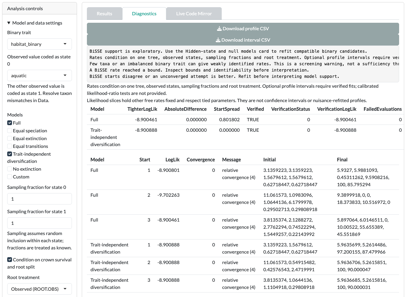
- Open Diagnostics before you look at Results.
Read the diagnostics
With the synthetic example, expect Diagnostics to open with warnings, including “A BiSSE rate reached a bound”. This is the app doing its job. Check these points before you trust any estimate:
- Bounds. A rate at its bound is not a reliable estimate. Look at which parameter hit the bound in Effective parameter constraints.
- Optimizer starts. Compare the log-likelihoods across starts. If starts disagree, refit before you interpret the result.
- Independent verification. Check that each model was verified by an independent optimizer.
- Data size. Few taxa or an unbalanced trait give weakly identified rates. A 19-tip example is small.
Profile uncertainty
After a fit, you can profile one rate:
- In Graph controls, choose the Model and Parameter to profile.
- In Analysis controls, open Profile uncertainty. Enter finite Profile lower search bound and Profile upper search bound values that enclose the estimate.
- Click Run profile uncertainty.
- Read the interval and profile grid in Diagnostics. An unresolved endpoint is shown as unavailable.
MuSSE
MuSSE extends BiSSE to 2 to 8 observed categorical states.
- Open the MuSSE card.
- Set Discrete trait to
locomotion_3state. - Click Fill state table and check the state-to-code mapping.
- Click Run MuSSE.
The number of parameters grows quickly with the number of states. For the state table format, see Custom input formats.
QuaSSE
QuaSSE links speciation and extinction to a continuous trait.
- Open the QuaSSE card.
- Set Continuous trait to
body_mass. - For practice, enter
10in Common measurement standard error. This is an invented value, not a biological measurement. - Click Run QuaSSE.
- Click Run grid and domain refits as an extra numerical check.
Check grid resolution, integration stability and optimizer verification in Diagnostics. With real data, you must justify any measurement error you supply.
Why weights may be withheld
Guane may show a finite likelihood but no model weight. It withholds weights unless the fits pass checks for convergence, repeatability, bounds and independent verification. The warnings in Diagnostics explain which check failed.
Compare AIC only within one card run. Do not compare AIC between the BiSSE, MuSSE, QuaSSE and hidden-state cards.
Before you interpret
- A BiSSE preference for trait-dependent rates can be produced by rate differences unrelated to the trait. Refit in Hidden-state and null models and compare against CID-2 and CID-4 before you interpret it.
- A trait-dependent rate is an association under the model, not proof that the trait caused diversification.
- Rates at bounds, disagreeing starts or failed verification mean the estimate is not reliable.
- Multistate hidden-state models, calibrated SSE tests and QuaSSE or hidden-state intervals are not available.
Read State-dependent speciation and extinction before you report.
Next step
Change the controls beyond the defaults in Advanced SSE models.