Advanced ancestral states

Set root priors, fix or constrain rate matrices, sample histories and posteriors, and add measurement error.

The worked example shows what a root prior does when the data carry no information.

You’ll learn What the root prior, fixed Q, optimizer bounds and sampling controls change, and how to spot a reconstruction that only echoes its inputs.
Time About 35 minutes
Prerequisites Ancestral state reconstruction tutorial; example loaded and matched in the Ancestral state reconstruction Data card

Scientific caution

The bundled example is synthetic. Its values are invented and its branch lengths are arbitrary. Results are a demonstration, not biological evidence.

Before you start

Load the example in the Ancestral state reconstruction Data card and click Use matched taxa. Resolve the mismatch shows each step. The Discrete traits and Polymorphic traits cards share one collapsed section, Advanced analysis controls. It is shown unless Framework is Bayesian Mk (sample rates).

Root and rate matrix

Root probabilities (pi)

Sets the prior probability of each state at the root.

Where: Discrete traits Advanced analysis controls Root probabilities (pi)
Default: Equal weights
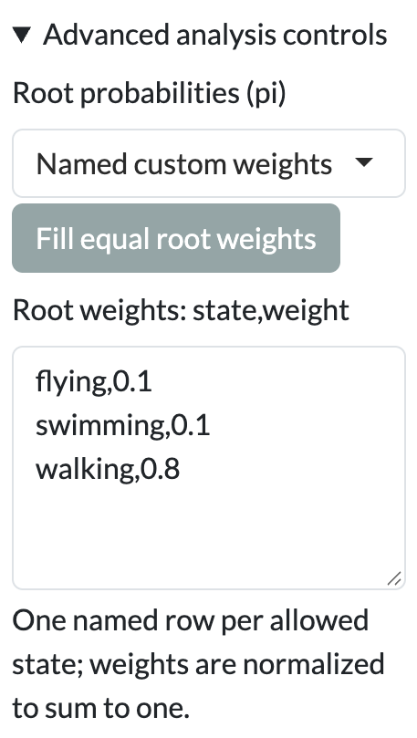
Change it when: You have independent evidence about the root state, for example from fossils or an outgroup. Choose Named custom weights, click Fill equal root weights, then edit the Root weights: state,weight box. See the root weights format.
Check after: The Effective settings preview is the exact R call Guane will run. Your weights are in its pi entry, written in R’s exact hexadecimal notation: 0x1.999999999999ap-4 is 0.1, and 0x1.999999999999ap-1 is 0.8. The plain check comes after the run: the root node’s row in the node probabilities table. If the root probabilities match your weights exactly, the data added nothing at the root.

Transition rates

Chooses whether Guane estimates the rate matrix or uses one you supply.

Where: Discrete traits Advanced analysis controls Transition rates
Default: Estimate rates
Change it when: You want to reconstruct under rates taken from another study or another fit. Choose Supply fixed Q, click Fill Q template from constraints, and edit the Fixed Q: named CSV matrix box. Untick Compare with ER, SYM and ARD: a fixed Q is not fitted, so there is nothing to compare. See the fixed Q format.
Check after: “Fixed Q must preserve the selected model rate-sharing constraints.” A fixed Q has no convergence to check; its rates are your assumption.

Optimization settings

Chooses the optimizer starts and exposes the rate bounds.

Where: Discrete traits Advanced analysis controls Optimization settings
Default: Guane: three deterministic starts, with Lower rate bound (min.q) 1e-10 and Upper rate bound 100
Change it when: Starts disagree, or a rate sits at a bound and you want to test whether the bound matters. Custom starting rates opens Starting rates (q.init); see the starting rates format.
Check after: The Optimizer starts graph in Results, and in Diagnostics: “A rate is near an optimization bound. Estimates and model rankings may be unstable.” or “Starting values reached different likelihoods”.

Custom rate constraints

An index matrix that says which transitions share a rate and which are forbidden.

Where: Discrete traits Model Custom Custom rate constraints
Default: Empty; start from Start custom matrix from and click Fill custom matrix
Change it when: ER, SYM and ARD do not match your hypothesis, for example when some transitions are impossible. See the custom rate constraints format.
Check after: The Transition-rate diagram in Results shows the rates you tied and forbade. Starts and bound warnings still apply.

Histories and posteriors

Number of histories

Sets how many stochastic character maps Guane draws. Mapping seed makes the draw repeatable.

Where: Discrete traits Framework Stochastic mapping (fixed fitted rates)
Default: 100 (range 2–500), with Mapping seed 999
Change it when: Sampled frequencies disagree with the analytic node probabilities. More histories reduce Monte Carlo error.
Check after: The Monte Carlo agreement plot in Diagnostics compares sampled frequencies with analytic probabilities. A very large request stops with “Requested mapping workload is too large”.

Gamma priors and proposals (CSV)

Sets a gamma prior and a proposal variance for each rate in Bayesian Mk.

Where: Discrete traits Framework Bayesian Mk (sample rates)
Default: Empty: gamma shape 1, rate 1 and proposal variance 0.1 for every rate. Click Fill rate-prior table for a template.
Change it when: You have prior information about rates, or chains mix poorly. See the rate prior format.
Check after: The chain tables in Diagnostics. “Split-Rhat exceeds 1.01 or is unavailable. Do not treat this run as converged.”

Continuous and polymorphic extras

Known standard-error column

Adds known measurement error to each tip.

Where: Continuous traits Use comparable marginal ML Known standard-error column
Default: None (zero error)
Change it when: Your table has a column of standard errors, on the same scale as the selected trait.
Check after: “Standard errors must be finite, nonnegative and on the selected trait scale.”

Ordered polymorphism

Allows only contiguous combinations in an order you give.

Where: Polymorphic traits Ordered polymorphism
Default: Off, with Maximum polymorphism 2
Change it when: The states have a natural order. Enter it in Constituent order (one state per line); see the constituent order format.
Check after: The Transition preview. The bundled example cannot be ordered: it has all three pairwise combinations.

Worked recipe

Worked example: your root prior, echoed back

Start in the Discrete traits card, with the example matched in the Data card.

Set Trait for reconstruction to locomotion_3state, Framework to Maximum likelihood and Model to ER.
Open Advanced analysis controls. Set Root probabilities (pi) to Named custom weights and click Fill equal root weights.
Edit Root weights: state,weight to flying,0.1, swimming,0.1 and walking,0.8. The Effective settings preview is the exact R call Guane will run. Your weights are in its pi entry, written in R’s exact hexadecimal notation: 0x1.999999999999ap-4 is 0.1, and 0x1.999999999999ap-1 is 0.8. The plain check comes after the run: the root node’s row in the node probabilities table.
Click Run Mk reconstruction. Open Diagnostics before Results.
Set Framework to Stochastic mapping (fixed fitted rates). Set Number of histories to 200 and Mapping seed to 42, then run again.
In Diagnostics, read the Monte Carlo agreement plot.

Expect the root pie to show exactly 0.1, 0.1 and 0.8, and every other node to show one third per state. Diagnostics warns “A rate is near an optimization bound. Estimates and model rankings may be unstable.” The fitted rates sit at the Upper rate bound of 100. The stochastic maps then show very many transitions on every branch, and their node frequencies agree with the analytic probabilities.

Advanced analysis controls open with named custom root weights flying 0.1, swimming 0.1, walking 0.8 — Advanced analysis controls with custom root weights.

Monte Carlo agreement plot comparing sampled node-state frequencies with analytic marginal probabilities for 200 histories — Sampled node frequencies agree with the analytic probabilities.

Saturated rates

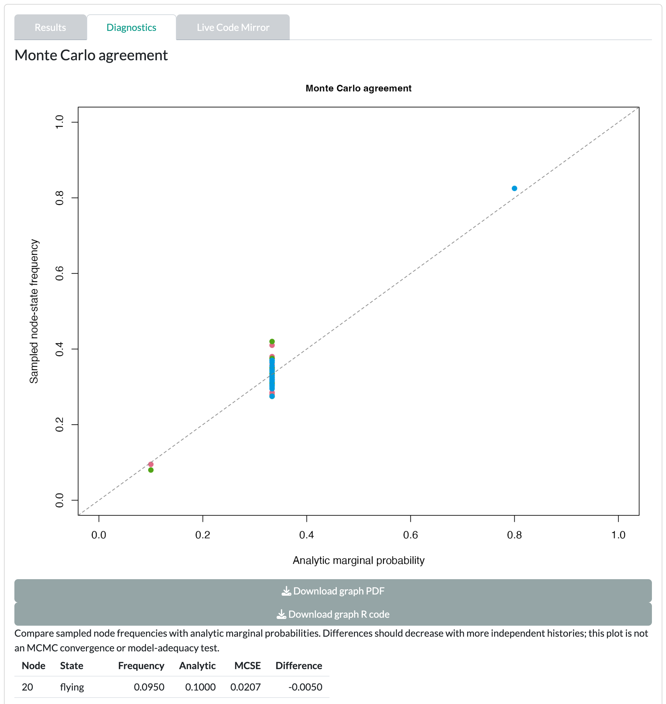
The root pie is the prior you typed, not information from the data. When a rate runs to its bound, states reshuffle along every branch, and the tips say nothing about their ancestors. Under ER, three of the four discrete example traits (habitat_binary, parental_care_binary and locomotion_3state) do this: their rate stops at the Upper rate bound of 100. diet_5state stops below the bound, so check its Diagnostics yourself instead of assuming it is informative. The model comparison table may still show weights; a model at a bound does not earn its weight. Treat this pattern as a diagnostic, not a finding.

Before you interpret

Scientific caution

If the root probabilities equal your prior, the data did not inform the root.
A rate at its bound is not an estimate, and weights for that model are not evidence.
A fixed Q is an assumption. Report where it came from.

Read Continuous ancestral reconstruction, Discrete and polymorphic ancestral reconstruction and Bayesian ancestral reconstruction before you report.