Ancestral state reconstruction
In this tutorial you estimate ancestral states for three kinds of trait: body_mass (continuous), locomotion_3state (discrete) and resource_use_polymorphic (polymorphic). Each estimate is conditional on the tree, the tip data and the model you choose.
The bundled example is synthetic. Its values are invented and its branch lengths are arbitrary. Results are a demonstration, not biological evidence.
Before you start
Open Ancestral state reconstruction, then its Data card. Load the example and click Use matched taxa. Resolve the mismatch shows each step.
Each card’s Framework menu lists Parsimony — planned. Parsimony is not available yet.
Continuous traits
- Open the Continuous traits card.
- Set Trait for reconstruction to
body_mass. - Set Framework to Maximum likelihood and Model to Brownian motion (BM).
- Click Run continuous reconstruction.
- In Results, switch Graph between Trait map, Phenogram, Node intervals and Selected node.
- Open Diagnostics and read any model warnings.
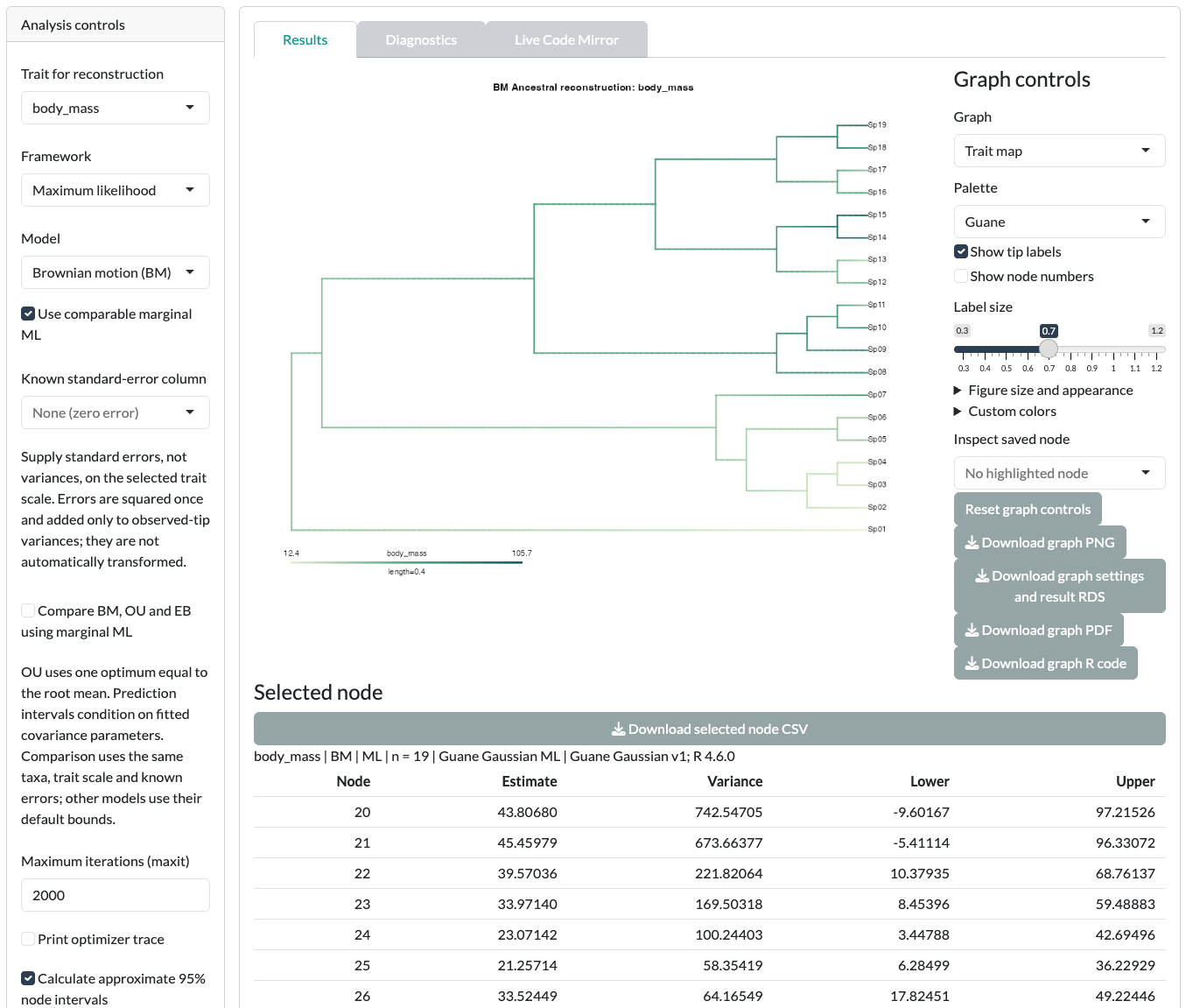
To compare models, tick Compare BM, OU and EB using marginal ML and run again. The comparison uses the same data and likelihood basis. OU and EB results need you to read their parameters and warnings; Guane may withhold intervals when they are unreliable.
For a Bayesian fit, set Framework to Bayesian BM. The card then shows MCMC controls, such as MCMC generations per chain and Chains, and posterior diagnostics.
Discrete traits
- Open the Discrete traits card.
- Set Trait for reconstruction to
locomotion_3state. - Set Framework to Maximum likelihood and Model to ER.
- Click Run Mk reconstruction.
- In Results, view the Node probability tree. Switch Graph to Transition-rate diagram to see the fitted rates.
- Open Diagnostics. Read the warnings and the model comparison before you interpret the pies.
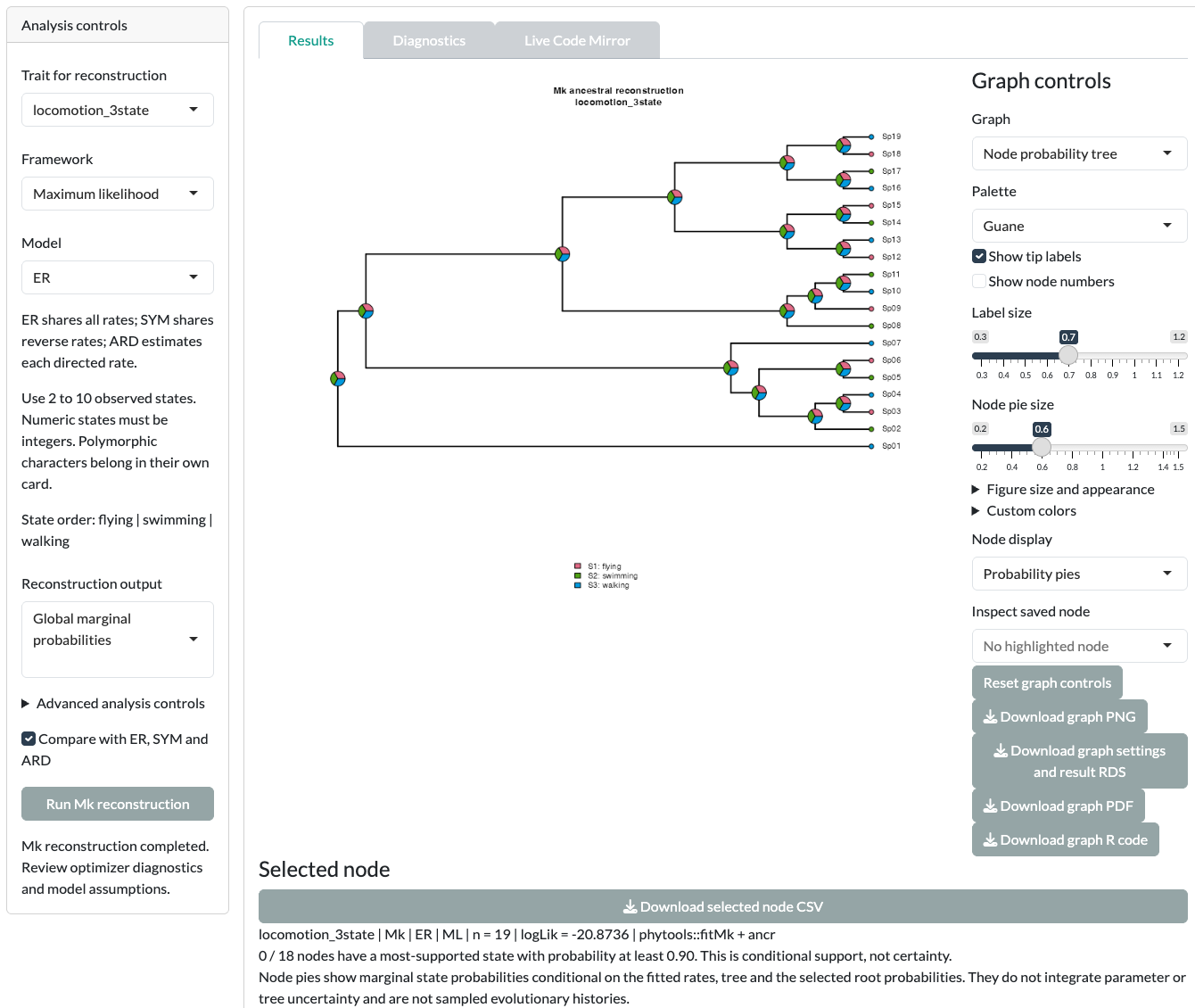
With the synthetic example, every node shows one third for each state. Results reports “0 / 18 nodes have a most-supported state with probability at least 0.90”. Diagnostics warns that “A rate is near an optimization bound”. The fitted ER rate has run to its upper limit. The model therefore treats the states as reshuffling along every branch, so the tips carry no information about their ancestors, and each node falls back to equal probabilities. This is an honest result, not a finding: do not read a pie’s largest slice, or the model weights, as evidence.
The Model menu also offers SYM, ARD and Custom. Advanced analysis controls hold root weights, optimizer settings and fixed rates. For custom matrices, see Custom input formats.
Two other frameworks answer different questions:
- Stochastic mapping (fixed fitted rates) samples histories conditional on the fitted rates and the tree.
- Bayesian Mk (sample rates) samples the rates themselves, with chain settings and diagnostics.
Polymorphic traits
A polymorphic value such as fruit+seed means both states coexist in the species. It is not uncertainty.
- Open the Polymorphic traits card.
- Set Trait for reconstruction to
resource_use_polymorphic. - Leave Ordered polymorphism off.
- Set Framework to Maximum likelihood and Model to ER.
- Read the Transition preview.
- Click Run polymorphic reconstruction.
Use unordered models with this example. It contains all three pairwise combinations, so no linear order can make every pair contiguous. An ordered analysis would reject it.
Node estimates, histories and interpolation
These outputs look alike on a tree, but they answer different questions:
| Output | What it is |
|---|---|
| Marginal node probabilities | Support for each state at one node, under the fitted model. |
| Joint ML assignments | The single most likely set of states across all nodes together. |
| Sampled histories | Possible histories drawn from the model, conditional on rates and tree. |
| Branch colors and phenogram lines | Interpolation between fitted node values. They are not observed trajectories. |
Use the method label shown with each result. Each card exports its graph as editable R code, PDF and PNG, and its data as CSV or RDS.
Before you interpret
- Every reconstruction is conditional on one tree, the tip data and the chosen model.
- Near-equal node probabilities mean the data do not resolve the state; they are not a finding.
- Sampled histories, marginal probabilities and joint assignments are different quantities.
Read Continuous ancestral reconstruction, Discrete and polymorphic ancestral reconstruction and Bayesian ancestral reconstruction before you report.
Next step
Change the controls beyond the defaults in Advanced ancestral states.