Skip to main content

Diversification

Plot lineages through time and fit diversification rate models to the bundled example tree.

In this tutorial you plot lineages through time (LTT) for the example tree. You then fit constant-rate models and see where the other rate cards fit. Diversification cards use the tree only.

• You’ll learn How to draw an LTT curve, fit Yule and birth-death models, and read a model comparison.
• Time About 20 minutes
• Prerequisites Guane running; example tree loaded in the Diversification Data card

Scientific caution

The bundled example is synthetic. Its branch lengths are in arbitrary units, not ages. Rates are per branch-length unit, not per year or per million years. Results are a demonstration, not biological evidence.

Before you start

Open Diversification, then its Data card, and click Load example data. These cards use the tree only, so you do not need to match taxa. See Example data and the Data card for what the example contains.

Lineage through time

An LTT curve counts the surviving lineages in a tree through its history. It is a description of the tree. It does not estimate speciation or extinction.

1. Open the Lineage through time card.
2. Leave Tree source set to Data tree.
3. Click Run LTT.
4. In Graph controls, change Time direction from Since origin to Before present, or tick Logarithmic lineage axis.

The LTT curve for the example tree. The time axis is in branch-length units.

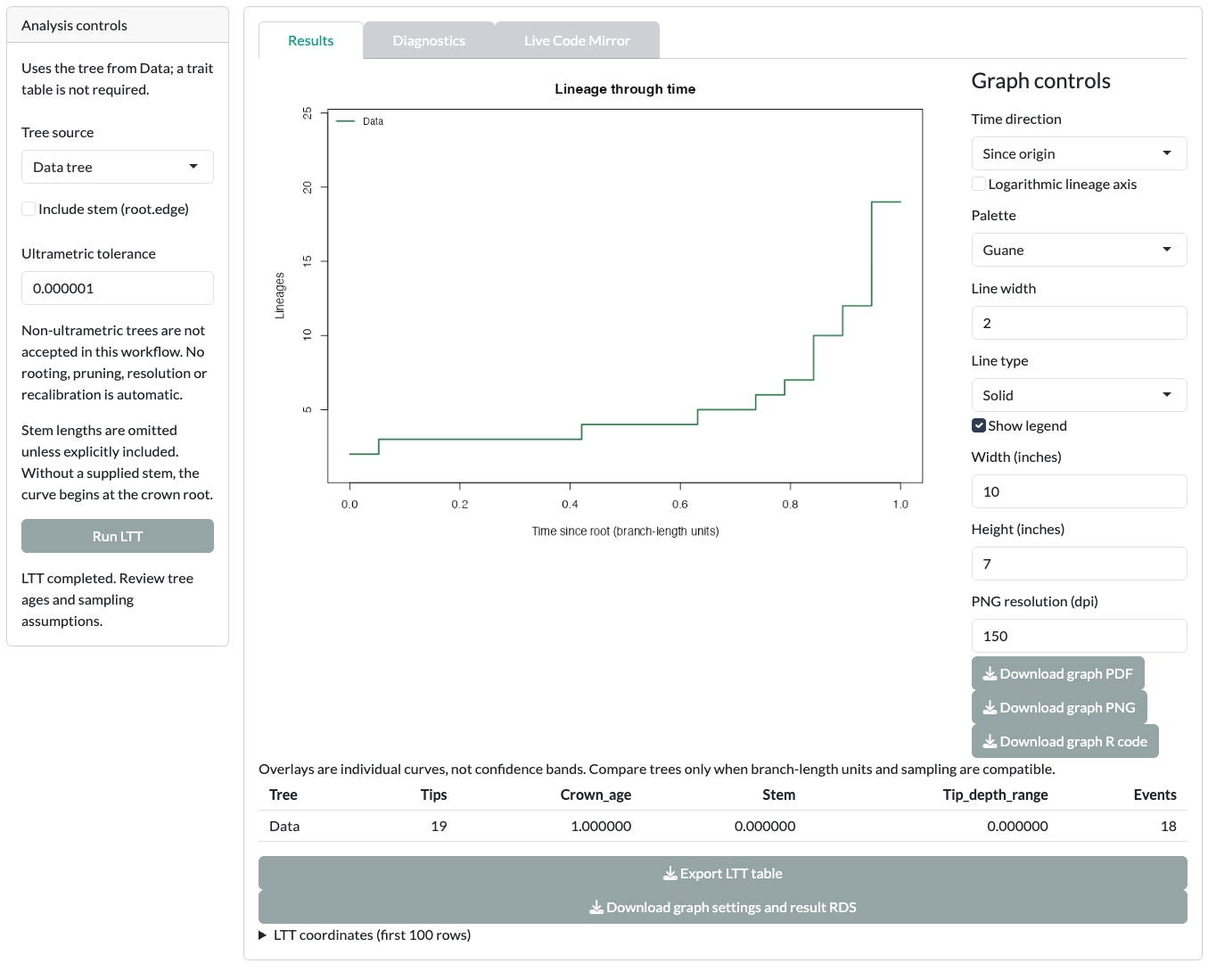
To overlay several trees, set Tree source to Uploaded tree set and upload up to 25 Newick files. Only overlay trees with comparable sampling and branch-length units.

Constant-rate models

1. Open the Constant-rate models card.
2. Under Models, keep both Yule (mu = 0) and Birth-death selected.
3. Click Run diversification models.
4. In Results, Graph starts at Rate estimates. Set it to Model comparison to see ΔAIC for each model.
5. Click Run uncertainty and diagnostics for profile likelihoods and conditional LTT checks.

The model comparison graph shows ΔAIC bars for the two fits.

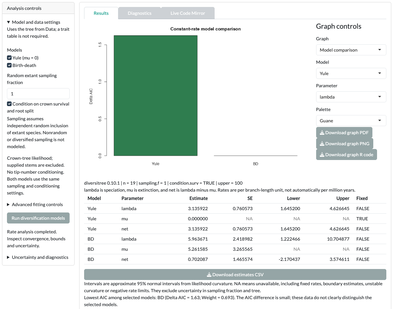
With the synthetic example, expect the app to say the data do not clearly distinguish the selected models. That is the honest reading: a 20-tip tree carries little information about extinction.

Other rate cards

Each remaining card answers a different rate question. Run each one the same way: set its options, click its run button, then read Results and Diagnostics.

Card	First run with the example	How to read it
Time-varying models	Keep the default candidates (Yule, BD, ExpYule, ExpBD). Click Run time-varying comparison.	View rates through time. Run time-model uncertainty adds profile, bootstrap and robustness checks. An exponential curve is a model assumption.
Clade-specific models	Choose non-overlapping Crown nodes with at least four tips each. Click Preview selected clades, then Run clade models.	Each clade is fitted separately. Compare models within a clade, not AIC across clades.
Joint clade-dependent models	Choose Joint shift nodes. Click Preview joint regions, then Run joint models.	One whole-tree likelihood with shared or shifted rates. Shifts sit at the base of the chosen branch.
Diversity-dependent models	Keep the default model. Click Run diversity-dependent models, then Run numerical diagnostics.	Curves relate rates to modeled diversity. Run uncertainty and robustness adds optional checks with more assumptions.

For every rate card, check failed starts, parameter bounds and numerical stability before you read estimates or model weights. Sampling fractions are taken as given. For clade and region sampling tables, see Custom input formats.

Before you interpret

Scientific caution

• Rates are per branch-length unit. The example tree is not dated.
• An LTT curve describes the tree; it does not estimate speciation or extinction.
• Extinction estimates from a small tree of living species are very sensitive to assumptions.

Read LTT and whole tree diversification, Clade dependent diversification and Diversity dependent diversification before you report.

Next step

Change the controls beyond the defaults in Advanced diversification.